Monday, May 12, 2014

Activity #13: Priory Navigation 2 + Paintball Guns

Introduction

This week, we were back at The Priory for a navigation exercise, but with a twist. All of the course markers from the last navigation exercise were in the same locations, and this time we had to navigate to all of the points (not just one of the three courses). Instead of using our map and compass for navigation, our groups (same groups as last time) had access to a shapefile that had the location of all the points. Using a GPS unit, we were to navigate to each point (in any order we wanted) and log a point with the GPS showing we had been there. The twist to this navigation assignment was that we all had paintball guns.

Since every group had different starting locations, and could navigate to the points in any order, groups would have random encounters with other groups. It was a navigation race, and if any member of your team was shot your whole team had to stop moving for 1 minute. The idea was to use geographical combat tactics to help better understand navigation. Do you want to walk straight through that clearing towards the course marker? Or take a little extra time going around so that you aren't ambushed without cover? The point of the game was to add another layer to our thought process (and make it really fun), instead of just traipsing through the woods from point to point.

Equipment


Trimble Juno GPS using ArcPad to track our progress and points.


Paintball guns. This Tippmann A-5 was the most common paintball gun we had access to, but there were several other random models in the bins as well.

Safety masks. This is not the one we used in the field, but I forgot to photograph the ones we used before they were put back in storage. The one pictured is the cheapest one I found on Amazon.com, and it looks to be drastically higher in quality than what our class was actually wearing.

Methods

On April 28, when we were supposed to do a navigation exercise at The Priory, the weather was pretty bad. Instead, that day was devoted to preparing for this last exercise on May 5th. This actually turned out to be good, as we had time to set up the GPS devices and export any layers and shapefiles we thought would help. We also planned out the path we would take once we started.

Figure 1 - Navigation map that would be used on the GPS. Contains
contour lines and a DEM. The red polygons show strict no-fire zones.
We had access to all of the data we had when we created our navigation maps for the last exercise (2 and 5 ft contour lines, DEM, navigation and point boundaries, and satellite imagery) as well as two new feature classes: no-shoot zones and the points we had to navigate to. Since we would only have the small screen of the Trimble to guide us, 2 ft contours would have been too cluttered. We went with 5 ft contours an an advance/retreat color scheme to help see elevation, the location points, and the no-shoot polygons (Figure 1). The no-shoot areas were in place because, while the woods surrounding The Priory were safe for this kind of activity, wearing masks and brandishing weapons near a building that houses a daycare center is typically frowned upon. We were under strict orders to not fire (or even look look slightly menacing) near these buildings.

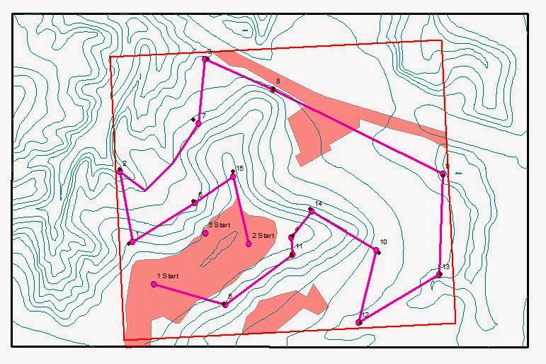
Figure 2 - Navigation map with the planned route.
Next we needed to decide the optimal path to take. Each group was given one of three starting points, as well as the first point we had to navigate to. The rest was up to us. Our group was given starting point 2 and a first nav point of 15. Figure 2 shows the path that we settled on. We kept terrain in mind and tried to plot a course that would be the quickest overall route, not just the next closest point. Lastly, we added an empty feature class where we could add the points we collected at each marker.


Figure 3 - ArcPad toolbar. 
To export the map to the GPS, we followed the same steps as in the microclimate assignment.On the ArcPad toolbar (making sure to have the ArcPad Data Manager extension activated under the Customize drop-down menu in Extensions), we clicked on the far left icon to Get Data for ArcPad (Figure 4). This created a map file that could be used in ArcPad on the GPS. The file with all of the data for ArcPad was saved on the computer, so I copy/pasted the folder into the GPS unit.

Figure 4 - Finished GPS map for use in The Priory.
Figure 4 shows the map in ArcPad. Notice that the background elevation raster image did not make it. I never did find our why that raster did not export, however it wasn't necessary since we had contour lines and already had an idea of terrain since the last time we were out there. We decided to just use the map as it was. With that, we were prepped and ready to start the activity. The navigation wouldn't happen until a week from then, so we just had to make sure that we checked out the same GPS unit the day of the activity.

Study Area


Figure 5 - Location and extent of our study area: The Priory.
On May 5th, our class met at The Priory. This study area was described here in the post for our first navigation exercise, and figure 5 shows the location of The Priory. The weather for this assignment was actually very similar to the last time we navigated these woods. It was a gorgeous, sunny day, though windy. We haven't had too many days yet this year that were sunny, warm, and dry all at the same time, so it was nice that both times we visited The Priory had these conditions.

Navigation

Before anything could be done, Professor Hupy and several students helped get all of the paintball equipment ready. Tanks of compressed gas and paintball hoppers had to be attached to all of the guns, and we tested them to make sure they all worked (Figure 6). By the time the entire class was there, the arsenal was laying on the grass near the edge of the woods (Figure 7).

Figure 6 - Professor Hupy and students assembling the guns
and making sure everything works. (Good trigger discipline, Joe) 

Figure 7 - All of the working paintball guns laying in the grass,
ready to go.

Figure 8 - The black circle shows where we encountered the
most resistance. Along that path we got into several firefights
with several different groups. The blue line shows the detour
we took around the fenced off area.
Once the equipment was ready, we all split up and went to our designated starting areas. The navigation itself was very simple. The map we created worked wonderfully, so we mostly just followed the path we created. We did have to make some detours, like the blue line around the no-fire zone in figure 8. This was fenced off and forced us to go around. Also, the black circle seemed to be where our group saw the most combat. This slowed us down and also caused us to deviate from the path in the process of tactical maneuvers.

I had the Trimble, so at each point I had to get close to the flag and collect a point. Jeremy and Zach covered me while doing this, since it took about 10 seconds to gather the point. Jeremy was the only one in our group wearing full camouflage, so during most encounters with other groups Jeremy would flank while Zach and I drew their fire.


Results

We were able to collect all the points, but we only finished 3rd. Figure 9 shows our navigation map again, but this time with all the points I collected.

Figure 9 - Completed navigation map with points we collected
at each marker.

Discussion

I was surprised that we only came in third. The first 3rd of our path included several firefights, but after that we rarely even saw another group, much less engaged them. I, for one, was getting exhausted in the heavy clothes, and I am not in as great of shape as many people in the class. The masks we had to wear was the biggest problem. My mask was constantly fogged up, so I could not see where I was walking or shooting. I had to constantly take it off and wipe the visor clean. This made me nervous, since the thought of getting shot in the face was not appealing. 

For each point I collected, I put the Trimble right under the marker. As you can see in figure 9, these points are not exactly on the points in the feature class given to us. This shows that, whether it was the GPS unit I was using or the one used to mark the points, GPS devices (even expensive ones) are not 100% accurate.

We had turned on a track log on the Trimbles. This would keep track of the actual path we walked the whole time. There was no track log when I retrieved the data, however. It turned out that the menu where we selected to activate the track log was actually just to display the track log, not turn it on. That was in a different menu. As a result, no one had this data. It would have been really interesting to see the path each group took, and to see how far we deviated from our path because of obstacles  or opposition.
 
Conclusion

Adding the paintball guns to the mix was more than just making it fun. After each firefight, we had to find out where we were and get back to our path. We had to plan the gathering of our points from a tactical perspective. One of the points (point 3) was just on the other side of a clearing. As we walked up to it, another group was approaching the same point from a different side of the clearing. Using cover fire and flanking, we had to suppress the other group long enough to gather the point and get out of there. It added another layer of problem solving to the navigation. Otherwise, we would have just walked through the clearing, taken the point, and moved on. With the threat of getting shot, we had to put the navigation part of the exercise to the back of our minds, making it second nature.

Tuesday, May 6, 2014

Activity #12: Priory Navigation 1


Introduction

The weather finally warmed up a little bit, so our class was able to do the navigation exercise that we created maps for back in Activity #5. For this activity, we were given a list of coordinates (in decimal degrees), along with elevation for each point. Using this list, the maps we created, and a compass, we had to navigate to each point and collect punches as proof that we had actually been there.

Here is a link to the blog post where I created the navigation map, for anyone too lazy to look at the sidebar.

Our class was split up into teams of three (the same groups we have been a part of for most activities) to navigate the course. There were three different courses set up in the priory, and two groups on each course.

Figure 1 - Visualization of azimuth.


To navigate by map and compass, we need to find the azimuth from where we are to the point we are trying to get to. Azimuth is an angular measurement of where something is in relation to true north and the observer. For example, north is 0° (or 360°), south is 180°, east is 90°, etc (Figure 1).


Study Area
Figure 2 - Image of The Priory taken from Google Earth.

The Priory (Figure 2), is the site of a former monastery that UW-Eau Claire purchased in 2011. It is 112 acres of mostly wooded land just south of Eau Claire (Figure 3). The building complexes at The Priory are still used as child care facilities and a nature academy, while the surrounding woods are used for recreation and educational purposes such as this class.

Figure 3 - Location of The Priory, and extent of our study area.
The day that our class went to The Priory for this activity was the most beautiful day so far this year. Temperatures were in the high 60s/low 70s and sunny. There were fairly strong northerly winds that day, but that wasn't really an issue once we were in the woods. This was outstanding, considering that the majority of field exercises our class has done this semester involved cold and/or sloppy weather. The class that did this assignment last year had to use snowshoes, so we certainly lucked out by being able to do this on a day that felt like summer.

The woods around the Priory had pretty think underbrush in some areas, which did make hiking through difficult at times. I had jeans and boots on, but several people in the class that were wearing shorts and t-shirts (since it was so nice out) came out with plenty of little cuts and scrapes.


Equipment


Figure 4 - The navigation map I created using a 50 x 50 meter grid system.
This is the map we plotted points on, as it has no background image or color.
Both 2 ft and 5 ft contour lines are used so that terrain can be easily
identified.


Figure 5 - The second map that we had was created by another
group member, Jeremy Huhnstock. This map utilizes aerial imagery
as well as 5 ft contour lines. This was helpful for visually identifying
landmarks, should we wonder off course and need to get our bearings.

Figure 6 - This is the compass that we used to navigate from one point to the next,
in conjunction with the maps.


Methods

Figure 7 - Coordinates for each point from the three different
courses.


To begin the exercise, each group was given a list of locations (Figure 7) and told which course they would be navigating. In our case, this was course 1. Using the coordinates given (which included both UTM and lat/long for each point), we had to plot the points on our map before we could start.
Figure 8 - Parts of a navigation compass.
With the points plotted on the map, and the Start point known, we could begin navigation. To navigate to the first point, the edge of the compass must be lined up between the point you currently at and the point you are trying to get to. Then, the degree dial is turned until the orienting lines are parallel with the north/south lines of the grid on the map (Figure 8). Once these are parallel, the number on the degree dial that is matched up with the direction of travel arrow will be the azimuth (or bearing) to the next point. Hold the compass level in front of you (keeping it away from any metal) and turn until the magnetic needle is inside the orienting arrow (sometimes referred to as "putting red in the shed"). You will then be facing the direction where the next point is located. 

Using the scale bar on the map, you can also get an approximate distance in meters to the next point. Using a pace count, (again, check back to exercise #5 to learn more) you can estimate distance traveled. In my case, I had about 67 paces (counting every other step) in 100 meters. When hiking over rougher terrain, however, your pace count will always be a bit more than when on flat pavement. The approximate distance can still be estimated, though.

With three people in a group, one person navigated using the map and compass, one person was a runner and the third person used pace count to keep track of distance. Once the navigator found the direction to the next point, the runner would run ahead to some landmark that was directly between the navigator and the point. Then the pace counter would follow, keeping track of distance. Finally, the navigator would catch up and repeat the process until we reached the point. Jeremy was the pace counter, I was the runner, and Zach was the navigator for this exercise.

Here is a short video that shows the basics of compass navigation.

Our group started by plotting the points for course 1 (Figure 9) on our map (Figure 10). Then, using the navigation techniques outlined above, we found our way to the first marker (Figure 11). This first one was relatively easy, as it was right near a trail. At each marker, there was a hole-puncher that we used on a laminated card to show that we had been to that location (Figure 12).

Figure 9 - List of points. Our group did course 1, the first set of points on the list.

Figure 10 - Map with points plotted (they are difficult to see in this picture).

Figure 11 - Finding the bearing to the first point.


Figure 12 - Laminated card used to punch at each location. This is after the first marker.
The second marker was slightly more difficult. It wasn't actually that hard to locate, but it was at the bottom of a steep ravine. Figures 13-15 are pictures from the bottom of the ravine while our group and another group were there punching our card.


Figure 13 - Marker #2, at the base of a ravine.

Figure 14 - The same ravine, facing northwest.

Figure 15 - Another view of marker #2.
Once we plotted a path to point 3, we realized that if we followed a straight line we would have to go up the steepest part of the ravine and then through another ravine on the way (Figure 16). Instead, we decided to hike out of the ravine at the easiest spot, then bypass the second ravine all together (Figure 17). To do this, we hiked out of the ravine at the southeast end, found our bearings to the tip of the other ravine, then found the azimuth again from there to point 3.
Figure 16 - The straight line path from point 2 to point 3. Notice
the steep terrain along this line.
Figure 17 - The blue line shows the path we decided to take.
We headed southeast up the easier part of the ravine. Then
headed towards point 3 while avoiding the second ravine.
Figure 18 - The third marker we went to, which
turned out not to be on our course.


This tactic did work quite well at first. The other group that was doing the same course as us took the straight-line path, and we overtook them while they were around the second ravine. Once we got to the marker, punched our card, and continued on to the next point, we realized that we had gone to the wrong marker. We had stumbled onto marker #7 by accident, and thought it was ours (Figure 18). Luckily, Professor Hupy and Zach Hilgendorf (who helped set up the course) were walking around the woods helping people out and noticed that we were headed the wrong way. They told us the markers were actually numbered so we would know if we were at the correct point.


Once our group found the point 3, it was pretty smooth sailing from there. We did not run into any other problems. Some of the points were relatively close together, so it was good that we found out the number was actually written on them. Otherwise we may have went to the wrong marker again.

Discussion

Since the map used a 50m x 50m grid, we had to estimate to some extent when plotting points. When we would navigate to a plotted point, we would have to walk in circles for a bit until we found the marker. However, using a smaller grid size, like 25m x 25m, would have made the map more difficult to read. Navigation would have probably been more difficult.

I was glad that I went with the 2 ft contours as well as the 5 ft contour lines for the map. When we decided to take an easier route out of the ravine, it was easy to spot the second ravine and knew to avoid it before we got to it. Even without any aerial imagery on this map, it was easy to read the topography and plan accordingly. I only wish I would have labeled the contour lines more evenly so elevation could have been figured out quicker.

Though Jeremy was the pace counter and I was the runner, we both ended up basically doing both. When Zach found the azimuth, Jeremy and I would both go out and both count our steps. This worked well for two reasons. Every so often, one of us would lose count, so it was nice to have another person counting as well. Second, since the only real 'landmark' the navigator could call out was "That tree over there...no, to your right...farther right...nope, back the other way..." it helped having two people out there to be the runner. Instead of having a navigator, runner, and pace counter, I thought it worked much better having a navigator and two runner/counters.

Despite having to backtrack to point 3, we still ended up being the first group to finish. It wasn't a race, but it was nice to know that our strategy worked pretty well.

Conclusion

Even if navigating by map and compass is something I never do again (though, I plan to do it much more in the future), it is a skill that every geographer (and possibly everyone in general) should at least have an introduction to. Having done this exercise already, navigating The Priory again with a GPS will be a lot easier. Not only have we already been out there and are more familiar with the area, but we also have a good geospatial understanding of the forest. I would like to make a topographical navigation map for

Monday, May 5, 2014

Activities #10 and 11: Aerial Mapping with a UAS

Introduction

Thanks to the ease in which people and organizations can share information and data over the Internet, aerial imagery for almost anywhere can be obtained through many different organizations or government entities. These images, however, may not always be the best option. Perhaps you want imagery for a very specific location or at a very specific time. Depending on what your project is, georeferenced images found online may not work. Using a UAS to collect your own images tailored specifically to your project may be the best way to go.

So far in this class, we have talked about and been introduced to UASs several times. This activity, which took place over two class periods, gave hands on experience using two different types of UAS: a multicopter and a balloon. In both cases, cameras attached to the UASs collected images of the surrounding area. It was up to us to mosaic these images together and georeference them so that the images would be correlated with their real-world locations and would be able to be used in programs like ArcMap.

Study Area


Figure 1 - Location of Eau Claire Sports Center
For both of these classes, our class returned to the Eau Claire Sports Center (Figures 1 and 2). This is the most convenient place to test UAS methods since it has several soccer fields, meaning there are few trees, electrical lines, or other obstacles that may cause issues with aerial devices. Plus, since we were doing these activites in early April, the soccer fields were not yet being used. We had a large, clear field all to ourselves.


Figure 2 - Eau Claire Sports Center. Notice how wide open the
area is. This is a great place to practice collecting aerial
images because there are very few obstacles.


Balloon


Methods


The balloon was inflated with helium in the parking lot of the sports center (Figure 3). Once filled, the picavet is attached to the line for the cameras to attach to. A picavet is a suspension-based rig that allows the cameras to stay relatively level with the ground, even if the balloon or kite is not (Figures 5 and 6). We used two different 12 megapixel cameras; one that produced images that were already georeferenced and one that did not. The cameras were set to collect a maximum of 300 images, capturing every 5 seconds.

Figure 3 - Inflating the balloon.

Figure 4 - Cody likes balloons.

Figure 5 - Attaching the Picavet.

Figure 6 - Picavet in action.


Figure 7 - Walking the soccer fields with the balloon in tow,
collecting aerial images.
The balloon was sent up to about 500 feet. At this height, the photos taken by the cameras would include a large area, and would overlap well when we mosaiced them later. As a class, we walked around the soccer fields taking turns holding the balloon (Figure 7). For the most part, we did not walk in any specific pattern, but we made sure that we covered as much area as we could. Only at one or two spots did we have to be careful of trees or power lines. For the most part, however, we didn't encounter any issues.

When we finished, the cameras were removed and the balloon brought down. Professor Hupy decided the most efficient thing to do with the balloon was to make it explode all over himself and the inside of a students car.

With the images taken, it was time to mosaic and georeference those images so the area as a whole could be analysed and the image could be used in programs like ArcMap. One of the students in our class, Drew Briski, was a huge help in this process. He was the first one to play around with the data and get it mosaiced together, and he taught the rest of the class what he learned. Here are the steps I followed for the next part of this post.

Figure 8 - All the tools needed to mosaic the images are
found in this menu, Workflow
There are several programs that be used to mosaic these images. I chose to use PhotoScan because Drew had such good directions for this program, and because images do not need to be georeferenced to mosaic them together. This can be done after in a different program. First I tried mosaicing images from the camera that georeferenced the images (Canon SX260), thinking that I would be able to skip that step then after I had my final TIFF. I only used about 25 images for this, since using all of the images would have taken several hours to process. Figure 8 shows the workflow menu in PhotoScan. Almost all of the tools I needed to use were in this drop-down menu. Add Photos, at the very top, is where you select the photos to use. Once those are added, I clicked Align Photos. This creates a point cloud of the images. Once that process was completed, Build Mesh was selected, which builds a TIN (triangulated irregular network) from the point cloud, followed by Build Texture. Once this is finished (Figure 9), the image can be exported as a TIFF file by going to File, Export Orthophoto. Since these images were already georeferenced, I brought the TIFF into ArcMap and ended there.
Figure 9 - Completed mosaic from the SX260 images. 

Figure 10 - 110 images from the Canon Elf mosaiced together.
After seeing the results, I decided to try the other set of photos from the Canon Elf. I used the same process in PhotoScan as I did with the previous set of images. This time, however, I used 110 photos to see how much better quality the results would be. Figure 10 shows the mosaiced image before I exported it as a TIFF.


Figure 11 - Georeferencing toolbar.
Since these images were not georeferenced when taken, the mosaiced image had no spatial reference. To georeference it, I brought it into ArcMap, added the georeferencing toolbar (Figure 11), and added the Imagery basemap so I would have a spatial reference to compare my TIFF to. On the georeferencing toolbar, I clicked the icon with the magnifying glass so that my unreferenced TIFF was opened in a different window. To add control points, the icon on the left (Figure 11) was selected.

Figure 12 - Adding control points in ArcMap.
Adding control points gives spatial reference to parts of the unreferenced image. For example, the first control point could be the corner of a house. I would click on that corner first on the unreferenced image, then on the same corner on the basemap. This tells the image that that is where that corner exists in real life. building corners, sidewalk corners, or other 90° angles always make great control points because they can be easily distinguished. The more control points you use, the more accurate the final image will be. Figure 12 shows an example of this. I used about 30 control points for this image.

Results


Figure 13 - Close up of the mosaiced image from the Canon Elf.
Figure 14 - Finished mosaic from the Canon SX260. Only
25 images were used for this one. This camera included
georeferencing for the images, but notice how off the image
is from the basemap below it.


Figure 15 - Finished mosaic from the Canon Elf. 110 photos
were used for this mosaic. This image I georeferenced myself
using control points in ArcMap.  Notice that this one is far
more accurate than the first try.


Discussion

The second mosaic using the Canon Elf turned out much better. This could simply be because I used 110 images instead of 25. That aside, the images that were already georeferenced were not very accurate. The camera was able to tell that the images were taken at the Eau Claire Sports Center, but that was about as close as it got. In the end, manually referencing the images proved to be much more accurate. Also, the images from the Elf were brighter and had much better contrast, making the finished product much better looking. Dealing with this one took much longer, however. It took a lot longer to mosaic, then I had to georeference it myself. When I brought the image into ArcMap, the image was mirrored, which made it difficult to add control points at first. But the image was correcting itself as I added more and more control points, so eventually looked correct.

Multicopter

Methods

Figure 16 - Joe's Y6 multicopter shown with remote control
and the laptop running Mission Planner.
While the end product (aerial photos of a specific area) is basically the same as using a balloon, the methods are quite different when using a rotary UAS. Since a balloon is fairly cheap, and can be operated by a single person, there isn't as much preparation that needs to go into it. A rotocopter, however, is a very expensive piece of equipment and, while it can be operated by a single person, should have a team of two or three people in control. For this assignment, Professor Hupy demonstrated with his own Y6 multicopter, shown in figure 16.

Figure 17 - Mission Planner software that has the checkpoints
and path for the Y6 to travel. On the left is a heads-up-display
that shows the altitude, pitch, and various other information
about the status of the Y6.


Before any mission, the mission must be planned out using a program that can communicate with the aircraft's on-board navigation system. There are many free, open-source programs that can accomplish this; in this case, we used Mission Planner (Figure 17). In this software, the path that the UAS travels is programmed using checkpoints over a map of the study area, as well as the elevation that the craft travels at. Both the checkpoints and elevation are extremely important so that the copter does not fly straight into a tree or a wall. When setting up the path, you have to know what the tallest obstacle in the are is so that you can set the elevation well above that. In this case, it was not too difficult since we were in an open field.

Figure 18 - Our class gathered around Joe Hupy
and his mobile command center (otherwise known
as a recycling bin).
Once everything was ready, the Y6 was launched. With Professor Hupy at the helm using his mobile command center (Figure 18), we watched the Y6 fly its course. Most rotocopters, including this one, have a battery life of only about 15-20 minutes. This limits how large of an area the UAS can cover. If it is a windy day, as it was the day we were using it, the battery life is even less since the craft has to use more energy to stay stable. The Y6 was not in the air for very long, but it was long enough to complete the path that Professor Hupy had programmed. After a few minutes of flight, the Y6 returned to the starting location and landed automatically.


Results

Figure 19 - One of the images taken by the Y6. Most of the
other images were unusable.


The results from the Y6 were not good, unfortunately. The images were very dark, and did not overlap well enough to be mosaiced. I tried mosaicing just like with the balloon data, and the result was just a dark blob. Figure 19 is one of the images taken, which is one of the best ones of the bunch.


Conclusion

Both the balloon and the Y6 had their pros and cons. As far as results, the balloon did much better than the multicopter. We got plenty of good, usable images from the balloon, but the Y6 didn't do very well. However, the image quality problem should be a small, easily fixed problem. The craft itself preformed exactly as planned. The Y6 flew an area of similar coverage as the balloon, but did it in under 15 minutes. It took us about 45 minutes to walk the fields, not counting the time it took to inflate the balloon and attach the cameras. The Y6 is more expensive and more complicated to operate, but is faster and under more control. The balloon is pretty cheap, and can still collect solid images, but is heavily influenced by weather and is far more time consuming.

The fact that we used a balloon at all was dependent on the weather. There was very little wind that day, but if it had been windy we would have used a kite instead. The Y6, and rotocopters in general, have far more practical uses. Consider if figure 19 was a house in an area experiencing severe flash flooding. Using a rotocopter to zip over areas and see where people are still trapped on rooftops would be extremely helpful, and it wouldn't put additional life in danger. That is not something you can do with a balloon. These assignments really showed the advantages and disadvantages of both types of UAS.

Used a balloon because it was not at all windy. If it was windy, we would have used a kite.
Simple technology- once it's up, just have to walk around, not much else you can do.

Thursday, April 10, 2014

Activity #9: Campus Mall Total Station Survey

Introduction

Figure 1 - Learning how to operate the Topcon
Total Station.
This exercise introduced our class to using the Topcon Total Station for doing topographical surveys. Each of our groups were instructed to survey an area roughly a hectare in size of anywhere on campus. Our class meeting on Monday consisted of learning how to set up and use the Total Station. In the classroom, we were shown how to set up and level the tripod and device. Then we went outside to learn how to gather data. From there, it was up to us to find times to meet as groups, check out equipment, and complete the survey.

The Total Station works by shooting a laser at a prism that is on top of a pole. The prism reflects the laser back and the Total Station can determine the location and topographical elevation by the angle of the laser and the time it took to travel. Typically, one person will hold the pole with the prism on it and one or two people will operate the Total Station. The person with the prism will stand in as many places as necessary to collect enough points.


Equipment

Topcon Total Station (Figure 2)
http://geoshack.com/wp-content/uploads/2011/03/GTP-3100W.jpg
Figure 2 - Topcon Total Station


Topcon GMS-2

https://www.uwec.edu/Geography/resources/images/GMS2_2.jpg
Figure 3 - Topcon GMS - 2


TruePulse 360 Laser Rangefinder
http://images2.opticsplanet.com/365-240-ffffff/opplanet-laser-technology-trupulse-360b-01.jpg
Figure 4 - TruePulse 360 Laser Rangefinder


Survey Area

Figure 5 - Location of UW- Eau Claire and study area.
Our group decided to do the new UWEC campus mall for our survey area (Figures 5 and 6). The aerial images are not up-to-date. The building within the red box in figure 6 was demolished and a new one constructed south of that location. The area within the red box is currently a grassy area with stone benches.

Originally, we wanted to do the same area of campus that we did for the distance azimuth survey. This area was too small and too crowded to do an effective survey, however. The campus mall is a wide open area that is more conducive to learning how to do our first survey.

The assignment called for surveying an area a hectare in size (100m x 100m). The area, however, did not get 100m in the north-south direction, so we extended the area east-west that we surveyed to get roughly the same area of coverage.

Figure 6 - Study area on campus. There are not yet any current
aerial images of campus. The area within the red box is an open,
grassy area with rock benches.


The following images (Figures 7- 10) are pictures of our study area.


Figure 7 - Facing north/northeast towards Schofield Hall

Figure 8 - Facing west/northwest towards McIntyre Library


Figure 9 - Facing southeast towards Roosevelt Ave.


Figure 10 - Facing southwest towards the Davies Center.


Methods

Figure 11 - Example of Total Station tripod setup.


To begin the survey, our group needed to set up and level the tripod as well as the Total Station itself. This would ensure that our measurements were accurate. The tripod legs need to be spaced equally apart and have a wide base to ensure stability (Figure 11).


Figure 12 - Leveling screw and circular level.


Next, the Total station can be placed on the tripod and screwed onto the top. Once the device is attached, it's time to level. There are two different areas to level: the circular level and the plate level. The circular level is calibrated by adjusting the length of the legs of the tripod until the bubble is in the center of the circle (Figure 12).


Figure 13 - Plate level.


Next is the plate level (Figure 13). There are three screws near the base of the device that can fine-tune the plate level (Figure 12). To get the bubble in the center of the plate level, face the device between two of the screws, turn one until the bubble is in the middle, then rotate the device to be in-between the next screws. Keep doing this until the bubble stays in the center of the plate level.


Figure 14 - Leveled Total Station ready to collect
data.


Once this step is done, both levels should be calibrated. Figure 14 shows a leveled, ready-to-go Total Station. The height of both the Total Station and the pole holding the prism are also measured and will be entered later.

First we used the GMS to gather a point directly below the Total Station. This would be used as our occupied point. The occupied point is the point that all the other data is collected from. If we have the location of this point, then everything we gather should be accurate (similar to the distance azimuth assignment we did earlier). We then had to set our backsight. We did this by using the TruPulse to find the azimuth to our backsight and label it as such in the GMS. We were then ready to start collecting data.


Figure 15 - Jeremy using the GMS to collect the points while I sight the
Total Station. Zach is circled in red holding the prism at the collection point.
For data collection, one of us held the pole with the prism at the point where data was being collected, one of us sighted using the Total Station, and the third group member used the GMS to record the data (Figure 15). We started in the corner of our study area nearest the library to the northwest and moved back and forth working our way towards the Total Station, then past it, to the southeast portion of our study area (Figure 16). Figure 16 also shows the points that we collected, 147 in total.


Figure 16 - The survey points that we collected, as well as arrows showing the direction and method of point collection.


Results

Our results seemed to be pretty accurate. It is difficult to tell in the figure 17 map (the aerial images are not up to date, so the Davies Center as well as Little Niagara Creek are not shown in the correct locations), but the area of lower elevation is where the campus mall slopes down to the creek. The rest of the survey area, while varying slightly, was mostly level.

Figure 17 - Results of survey interpolated using the Nearest Neighbor method. Range of elevation is from 236.263 - 239.263 meters above sea level.

Discussion

The difficult part of this exercise was setting up the total station. Our professor came out with us when we went to do the survey to show us how to navigate the menus and set up the device. The actual data collection was simple and just a matter of doing the same thing 147 times. The largest issue we encountered (and from talking with others, we weren't the only group that did) was that the Bluetooth connection from the Total Station to the GMS kept disconnecting. This was pretty frustrating, and we never really found out why this was happening. We just had to go back into the settings, reconnect, and continue.

We had intended to switch off roles so everyone got some experience with each, but we realized that the survey went quicker if we each did the same thing for the duration. We were able to get into a good rhythm that way, instead of trading off and having to get into a new rhythm each time. Also, when we leveled the Total Station, we did not take into account that the three of us are different heights. I started off as the one sighting through the device, and I am the shortest one in the group. Zach is much taller than I, and it would have been uncomfortable for him to have to bend over the whole time. We could have adjusted the station, but that also would have taken more time. While it was mostly sunny that day, there was a chilly wind. We decided to not break our momentum and finish the project as quickly as possible.

Luckily, we had no issues when exporting the data to the computer. It went smoothly, as did interpolation and map creation.

Conclusion

The results, while accurate, are a little boring to look at. There is only about a 3 meter range between the highest and lowest point, meaning the survey area was pretty level. This worked out well since we all were using this technology for the first time. Learning would have been slightly more difficult had we had a very diverse terrain. But a slightly greater elevation range would have at least made the resulting map more satisfying.

Terrain surveying is something that is always needed in various different work sectors. I like having a general understanding of the processes, but I hope to gain more knowledge in the future. When surveying larger plots and more dynamic terrain, the Total Station would have to be moved, adding extra steps to the process. This activity was only a brief introduction to land surveying.